Oct 10, 2023
3m read
Run Jupyter Notebooks on a GPU on the Cloud#
GPUs accelerate tasks like ML training, computer vision, and analytics, but can be challenging to access. Using the cloud can open up access to GPUs, but comes with its own challenges including:
Complex Cloud Infrastructure: AWS SageMaker, for example, requires navigating AWS IAM roles, VPC settings, and other cloud configuration steps before even starting a GPU instance.
Limited Customization: Tools like SageMaker and Google Colab provide managed environments, but they can feel restrictive, making it hard to install custom dependencies or optimize GPU usage.
Poor Developer Experience: Compared to tools like Jupyter Notebooks, the UI for SageMaker or Colab can feel clunky and unintuitive, adding friction to the development process.
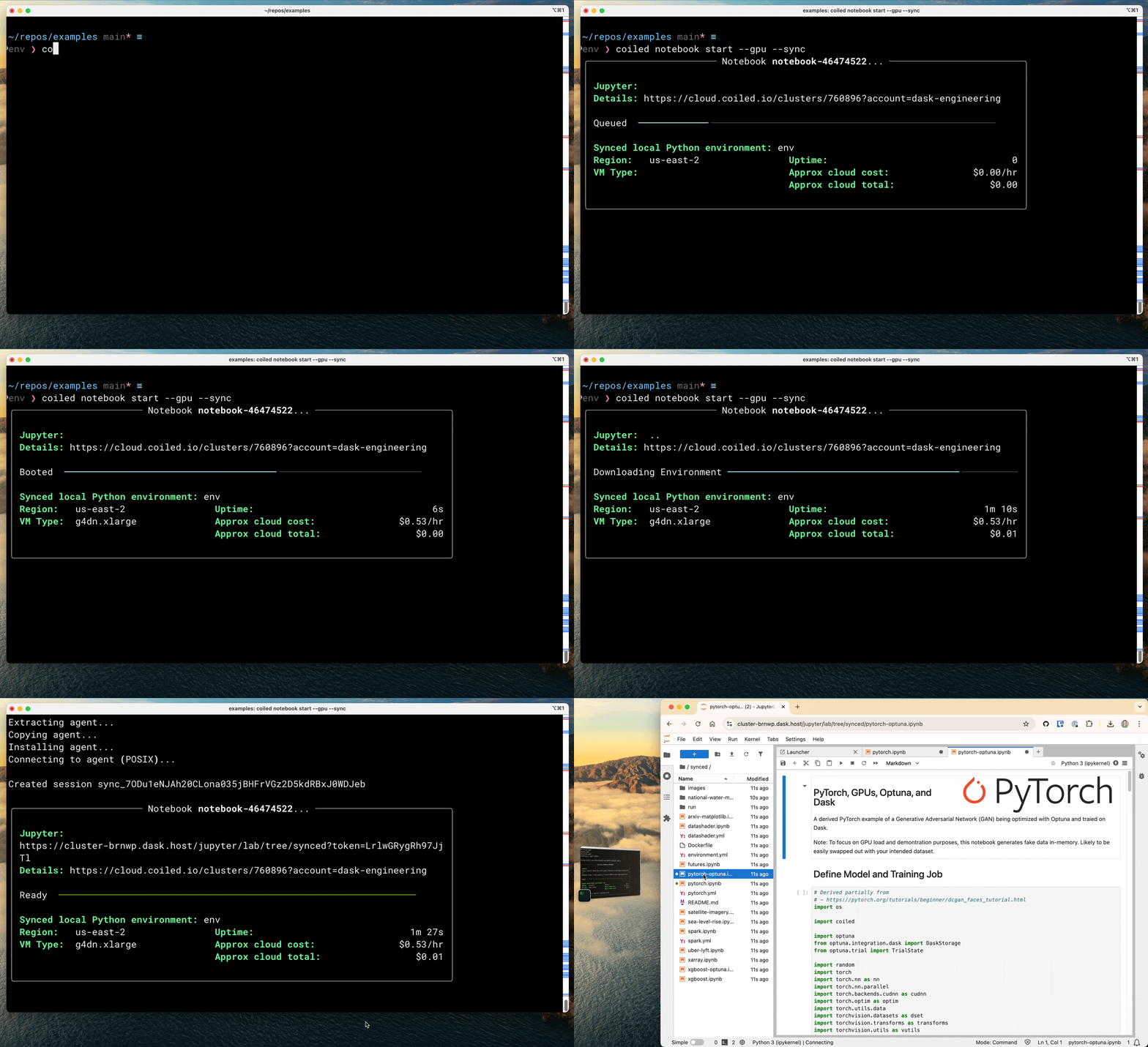
Coiled can launch a GPU-enabled Jupyter Notebook for you, from your own AWS, GCP, or Azure account, in a couple minutes.
$ coiled notebook start --gpu --sync

This has a few benefits:
GPU access: You’ll get temporary access to a GPU machine for as long as the notebook is running. When you’re done, it’ll turn off to minimize costs.
Software synchronization: You’ll get all of your current Python packages, including the same version of libraries like PyTorch, but those libraries will be properly configured (with CUDA drivers and everything) to operate on the underlying GPU. You don’t need to mess around with Docker.
File synchronization: You’ll also get all of your local files, including your notebooks, live-synced up to the cloud machine running Jupyter. Additionally, any changes you make in the notebook on the cloud machine will be synchronized back down to your computer, saving all of your changes on your local hard drive.
This creates a seamless experience for interactive work.
Getting Started#
If you haven’t already signed up for Coiled, it’s easy to get started. You’ll get 500 free CPU hours each month, though you’ll still have to pay your cloud provider.
Next, install Coiled alongside additional notebook dependencies like jupyterlab and your machine learning library of choice.
$ conda create -n env python=3.11 pytorch torchvision coiled jupyterlab jupyter-server-proxy
$ conda activate env
$ pip install "coiled[notebook]" torch torchvision
Then start a JupyterLab instance on a GPU-enabled VM on the cloud:
coiled notebook start --gpu
Under the hood, Coiled handles:
Provisioning a cloud VM with GPU hardware. In this case, a g4dn.xlarge (Tesla T4) instance on AWS.
Setting up the appropriate NVIDIA drivers, CUDA runtime, etc.
Automatically installing the same packages you have locally on the cloud VM.
Making sure to install the CUDA-compiled version of PyTorch on the cloud VM.
You can also include additional arguments like:
--syncto live-sync your local files, including your Jupyter Notebooks, to the cloud machine. Any changes you make in the notebook running remotely will be synchronized back down to your computer. You’ll need Mutagen installed.--vm-typeto request a specific VM type.--containerto specify a Docker container.--regionto specify a region. We find GPUs are often easier to get in AWS regionus-west-2.
See our documentation for more details.
Example: Define a PyTorch Model#
Now that we have a notebook running, we can define a PyTorch neural network and use it for model inference. We’ve adapted this example from this introductory PyTorch tutorial.
import os
import torch
from torch import nn
from torch.utils.data import DataLoader
from torchvision import datasets, transforms

# Select what hardware to use
if torch.cuda.is_available():
    device = torch.device("cuda")        # NVIDIA GPU
elif torch.backends.mps.is_available():
    device = torch.device("mps")         # Apple silicon GPU
else:
    device = torch.device("cpu")         # CPU
print(f"{device = }")

class NeuralNetwork(nn.Module):
    def __init__(self):
        super().__init__()
        self.flatten = nn.Flatten()
        self.linear_relu_stack = nn.Sequential(
            nn.Linear(28*28, 512),
            nn.ReLU(),
            nn.Linear(512, 512),
            nn.ReLU(),
            nn.Linear(512, 10),
        )

    def forward(self, x):
        x = self.flatten(x)
        logits = self.linear_relu_stack(x)
        return logits
We can then use the model to generate predictions based on the input data.
model = NeuralNetwork().to(device)

X = torch.rand(1, 28, 28, device=device)
logits = model(X)
pred_probab = nn.Softmax(dim=1)(logits)
y_pred = pred_probab.argmax(1)
Next steps#
This example was primarily illustrative, to show how you can get up and running with Jupyter Notebooks on GPUs. For more extensive machine learning examples you might consider: