Processing a 250 TB dataset with Coiled, Dask, and Xarray
We processed 250TB of geospatial cloud data in twenty minutes on the cloud with Xarray, Dask, and Coiled. We do this to demonstrate scale and to think about costs.
Many people use Dask with Xarray to process large datasets for geospatial analyses, however, there is pain when operating at a large scale. This comes up in a few ways:
Large task graphs due to too-small chunks causing the scheduler to become a bottleneck
Running out of memory due to one of:
Dask being too eager to load in data
Rechunking
Unmanaged memory
Too-large chunks
Many of these problems are now fixed (e.g. too-eager data loading), but not all. We wanted to run a big-but-simple Xarray problem to experience this pain ourselves and demonstrate feasibility. We’re also interested in optimizing costs, so we decided to play around with that too.
In this example we’ll process 250 TB of data from the National Water Model, calculating the ground saturation level in every US county. The calculation will take ~20 minutes and cost ~$25.
National Water Model Dataset
The National Water Model (NWM) is a complex hydrological modeling framework that simulates observed and forecasted streamflow across the US at a fine spatiotemporal scale. Many organizations use the NWM to make decisions around water management and to predict droughts and flooding. For more background, read America Is Draining Its Groundwater Like There’s No Tomorrow from The New York Times, published just last week.
In this example, we use a dataset from a 42-year retrospective simulation available on the AWS Open Data Registry. These historical data models provide context for real-time estimations and as a historical baseline for training predictive models.
We calculate the mean depth to soil saturation for each U.S. county:
Years: 1979-2020
Temporal resolution: every 3 hours
Spatial resolution: 250m grid
Data size: 252 terabytes
Processing one year of data
We first run this computation for one year (drawn from this example by Deepak Cherian). We process 6 TB of data, which takes about 8 minutes and costs $0.77 on a Coiled cluster with 40 workers, each with 16 GiB of memory. You can run this example yourself in our documentation. This analysis produces the plot below:
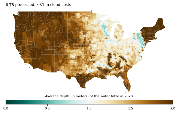
Since this is only a subset of the full dataset, we thought it’d be fun to run this for the full 42 years rather than just 1.
Scaling up to the full dataset
We now run this computation on all 42 years of the 250 TB dataset. This takes 24 minutes and costs $25 using 200 workers each with 64 GiB of memory. You can see the example here.
This presents a few challenges at first:
Large task graph (~344 MB)
Running out of memory (and spilling to disk)
Unnecessary rechunking
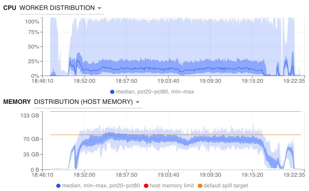
Median CPU usage is low with a large range. Memory usage is high and consistently spilling to disk, which significantly slows runtime.
So we make a few adjustments.
Larger chunk sizes
By default each chunk size is 200 MiB, resulting in a Dask graph of 1.3 million chunks. By increasing the chunksize to 840 MiB, we reduce the Dask graph to 320k chunks:
ds = xr.open_zarr(
    fsspec.get_mapper("s3://noaa-nwm-retrospective-2-1-zarr-pds/rtout.zarr", anon=True),
    consolidated=True,
    chunks={"time": 896, "x": 350, "y": 350}
)
Memory-optimized VMs
We further improve memory usage with memory-optimized instance types with a higher memory to CPU ratio. Since peak RAM was ~20 GB, we use r7g.2xlarge:
cluster = coiled.Cluster(
    ...,
    scheduler_vm_types="r7g.xlarge",
    worker_vm_types="r7g.2xlarge",
)
Launch from a remote VM
Lastly, we use Coiled Run to submit this workflow from a VM in the cloud to speed up uploading the task graph to the scheduler.
coiled run --region us-east-1 --vm-type m6g.xlarge python xarray-water-model.py
Dask uploads the task graph from the client to the scheduler, and if this were running locally we’d be relying on home internet speeds (which aren’t bad for me in Seattle, but this step helps speed things up a bit).
Results
This improves runtime and CPU- and memory-utilization quite a bit.
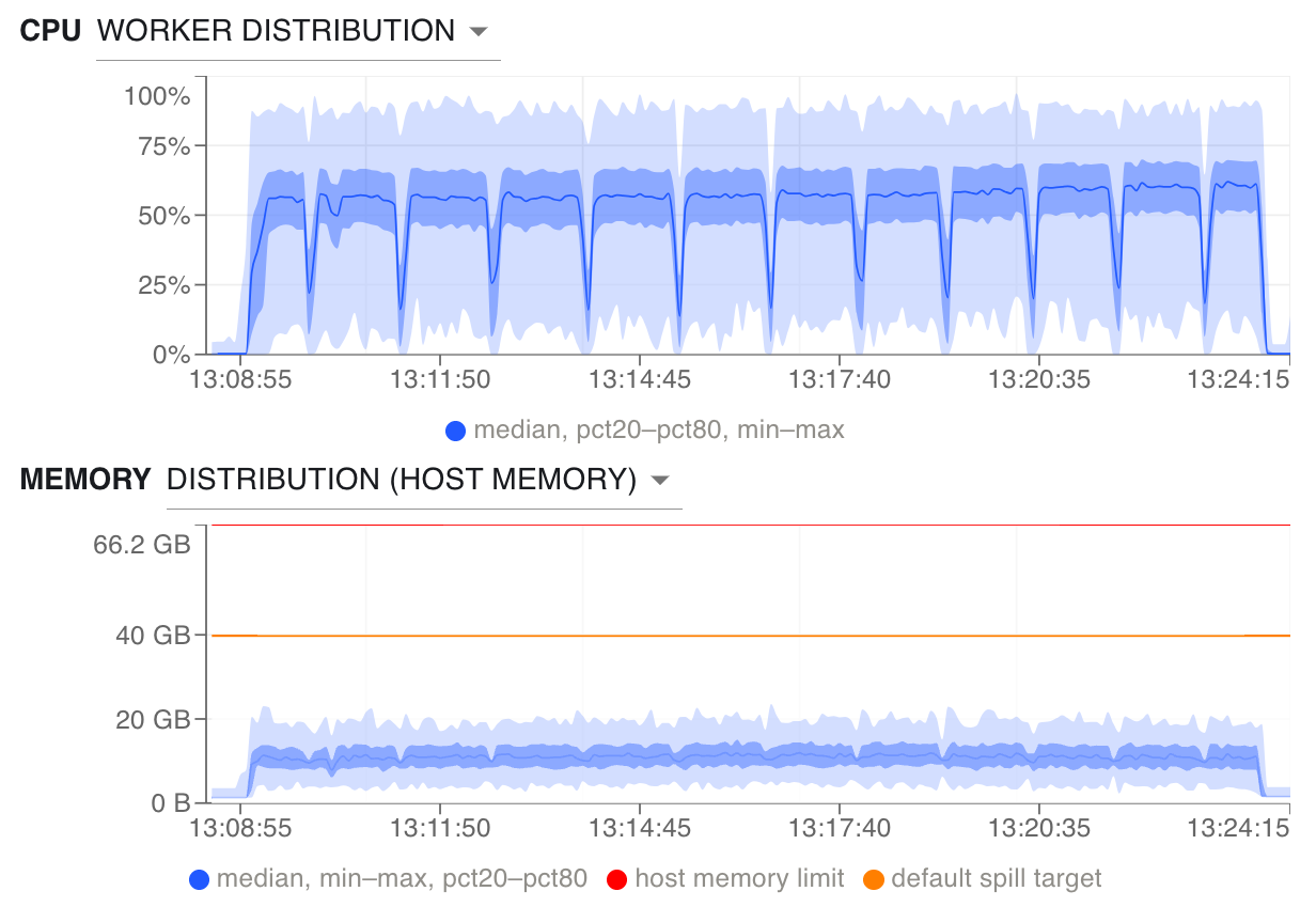
Median CPU usage is much higher at ~55%. Memory usage is consistently between 5 and 20 GB and we’re no longer spilling to disk.
Optimizing costs
In addition to trying to improve performance, we also want to optimize costs. There are a few ways we do this:
Use spot instances, which are excess capacity offered at a discount.
Use ARM-based instances, which are less expensive than their Intel-based equivalents, often with similar, or better, performance.
Use a region close to our data to avoid egress charges.
cluster = coiled.Cluster(
    region="us-east-1", # choose region close to data
    worker_vm_types="r7g.2xlarge", # ARM
    compute_purchase_option="spot_with_fallback" # spot instances, replaced with on-demand
)
We save $25 by using r6g ARM-based instance types rather than the x86-based equivalent. This is in part because runtime is nearly 10 minutes faster for the ARM-based instance types (others have similar findings).
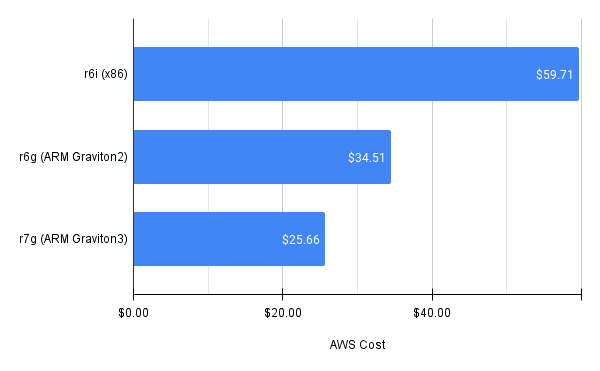
Comparing r6i x86-based vs. r6g and r7g ARM-based EC2 instance types.
We also use more spot instances, since r6g instances have a much lower frequency of spot interruption than r6i (<5% vs. >20%, respectively). Switching to the newer r7g ARM Graviton3 instances saves us an additional $9, mostly due to a faster runtime of ~6 minutes.
Conclusion
We ran a large Xarray workflow with three goals in mind:
Demonstrate feasibility
Expose rough edges at scale
Explore cost dimension of these problems.
Mission accomplished. We processed a quarter-petabyte for $25.
We also found opportunities for optimization like large graph sizes, chunksize tuning, and hardware choices. We hope this article helps point others in this situation in good directions. It’s also helping to inform the internal Dask team’s work prioritization for the coming couple of months.
In the future we’d like to run similar calculations, but with a more complex workflow (like rechunking). We hope that that exposes even more opportunities for optimization.
Want to try this experiment yourself?
Download the notebook to run one year or the script to run all 40 years.
Follow the Coiled setup process (this runs comfortably within the Coiled free tier). You can also find Coiled on AWS Marketplace.