Feb 5, 2024
4m read
One Trillion Row Challenge#
Sarah Johnson
Last month Gunnar Morling launched the One Billion Row Challenge with the task of writing a Java program for retrieving temperature measurement values from a text file and calculating the min, mean, and max temperature per weather station. This took off greater than anyone would expect, gathering dozens of submissions from different tools.
We joined in the fun and made our own unofficial Python submission for Dask, which ran in 32.8 seconds on a MacBook. Fellow Dask maintainer Jacob Tomlinson took things a step further, and ran the challenge on GPUs in 4.5 seconds.
This got us thinking, what about a trillion row challenge? The 1BRC was fun, and it’d be interesting to compare performance across different sets of big data tools at a much larger scale.
How can you participate?#
Your task is to use any tool(s) you’d like to calculate the min, mean, and max temperature per weather station, sorted alphabetically. The data is stored in Parquet on S3: s3://coiled-datasets-rp/1trc. Each file is 10 million rows and there are 100,000 files. For an extra challenge, you could also generate the data yourself.
Open an issue in the 1TRC repo with your submission and enough details for someone else to be able to run your implementation. This includes things like:
Hardware
Runtime
Reproducible code snippet
There is no prize and everyone is a winner. Really, the idea is to solicit ideas and generate discussion.
The next sections dive into the dataset generation process in more detail and an example of running the challenge using Dask.
Data Generation#
Our goal is to make the dataset easy for you to generate yourself, but also easy to access if you don’t have many TBs of data storage available. Using the 1BRC dataset as a template, we scaled up to one trillion rows, and wrote the data to Parquet on S3 (thanks to Jacob Tomlinson for the data generation script).
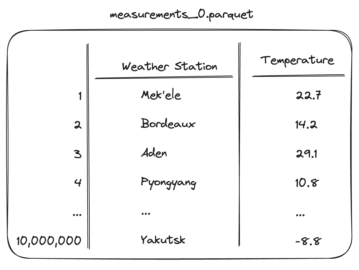
You’ll be working with 100,000 Parquet files, each with 10 million rows. The dataset is accessible on S3: s3://coiled-datasets-rp/1trc.#
Here’s what you’ll be working with:
100,000 Parquet files. Each files has 10 million rows and is 24 MiB on disk, for a total of 2.5 TiB.
Stored on S3
s3://coiled-datasets-rp/1trc. This is a requester-pays bucket in AWS region US East (N. Virginia). Those using AWS can avoid incurring charges by reading in the data from a cloud VM that’s also running inus-east-1.
Choosing good chunk sizes#
The first decision was how to split up a trillion rows of data. There’s not really one right answer here. You need small enough chunks that many could fit on a single worker’s available memory at one time. If the chunks are too small, this could mean an unnecessarily large task graph. If the chunks are too big, then you would be limited to specific high-memory machine types or risk running out of memory. For Dask, this usually means starting with somewhere around 100–500 MiB memory usage per chunk (note, this is when loaded into memory, not the size on disk).
If you read a single file into memory, it takes up ~228 MB, which is a good place to start.
import dask.dataframe as dd

df = dd.read_parquet(
    "s3://coiled-datasets-rp/1trc/measurements-0.parquet"
)
df.info(memory_usage=True)
<class 'dask.dataframe.core.DataFrame'>
Columns: 2 entries, station to measure
dtypes: float64(1), string(1)
memory usage: 228.5 MB
CSV vs. Parquet#
We first tried to use text files, but found Dask to be prohibitively slow at this scale. We generated 100,000 CSVs, each 131.6 MiB on disk for a total of 12.5 TiB. Creating the task graph for 1,000 files took ~30 seconds. There is certainly more we could dig into here, but we decided using Parquet is more realistic for working with this scale of data.
CSVs are everywhere and fine solution if you’re not working with much data. Parquet is more performant, though, especially if you have large datasets. This is in part because Parquet is more compact to store and faster to read. Since we’re processing a lot more data than the 1BRC, it makes sense to use Parquet.
Storing data on S3#
The dataset is publicly available on AWS S3 in s3://coiled-datasets-rp/1trc in AWS region US East (N. Virginia). The dataset is publicly available in a requester-pays bucket, which means you don’t have to worry about storing the data, but you are responsible for any data transfer or download costs (more details in the AWS documentation).
If you’re using AWS, you can avoid data transfer costs by running your computation in us-east-1, the same region as the data.
1TRC with Dask#
Here’s an example of how we ran this challenge using Dask and Coiled. It took 8.5 minutes and cost $3.26 in AWS cloud costs (10 minutes if you include cluster start time).
import dask_expr as dd
import coiled

cluster = coiled.Cluster( # Start Coiled cluster
    n_workers=100,        # 100 m6i.xlarge instances
    region='us-east-1',   # Faster data access and avoid data transfer costs
)
client = cluster.get_client()

df = dd.read_parquet(
    "s3://coiled-datasets-rp/1trc/",
    dtype_backend="pyarrow",
    storage_options={"requester_pays": True}
)
df = df.groupby("station").agg(["min", "max", "mean"])
df = df.sort_values("station").compute()
Similar to the 1BRC submission, most of the time is spent in I/O, in this case on read_parquet. Looking at the task stream it seems the cluster resources are well utilized, since there’s little white space.
Dask dashboard during the 1TRC, most of the time is spent on read_parquet tasks (yellow).#
Optimizing costs#
Processing 2.5 TB cost us $3.26. This is cheap. We can bring the cost down ~3x to $1.10 by:
Using Spot instances, which are excess capacity offered at a discount.
Using ARM-based instances, which are less expensive than Intel-based equivalents with the similar, or better, performance.
cluster = coiled.Cluster(            # Start Coiled cluster
    n_workers=100,                   # 100 m7g.xlarge instances
    region='us-east-1',              # Faster data access and avoid data transfer costs
    arm=True,                        # Use ARM-based instances
    spot_policy="spot_with_fallback" # Use spot, when available
)
In addition to being less expensive, using more performant ARM-based instances lowers computation runtime to 5.8 minutes (8 minutes if you include cluster start time).
Conclusion#
Looking forward to seeing all your challenge submissions in the 1TRC repo. Thanks to Jacob Tomlinson for helping kick things off (looking forward to seeing a GPU implementation soon).