Perform a Spatial Join in Python

This blog explains how to perform a spatial join in Python. Knowing how to perform a spatial join is an important asset in your data-processing toolkit: it enables you to join two datasets based on spatial predicates. For example, you can join a point-based dataset with a polygon-based dataset based on whether the points fall within the polygon.

	GeoPandas	Dask-GeoPandas
Perform Spatial Join
Support Geographic Data
Parallel Processing
Larger-than-memory Datasets

In this blog, we will use the New York City Taxi and Limousine Commission dataset to illustrate performing a spatial join in Python. We will join the taxi pickup location of each individual trip record to the NYC neighborhood it is located within. This will then allow us to bring in public health data at the neighborhood level and discover interesting patterns in the data that we could not have seen without performing a spatial join.

Spatial Join: Different Python Libraries

There are several different ways to perform a spatial join in Python. This blog will walk you through two popular open-source Python you can use to perform spatial joins:

1. Geopandas

2. Dask-GeoPandas

Dask-GeoPandas has recently undergone some impressive changes due to the hard work of maintainers Joris Van den Bossche, Martin Fleischmann and Julia Signell.

For each library, we will first demonstrate and explain the syntax, and then tell you when and why you should use it. You can follow along in this Jupyter notebook.

Let’s jump in.

Spatial Join: GeoPandas

GeoPandas extends pandas DataFrames to make it easier to work with geospatial data directly from Python, instead of using a dedicated spatial database such as PostGIS.

A GeoPandas GeoDataFrame looks and feels a lot like a regular pandas DataFrame. The main difference is that it has a geometry column that contains shapely geometries. This column is what enables us to perform a spatial join.

Sidenote: geometry is just the default name of this column, a geometry column can have any name. There can also be multiple geometry columns, but one is always considered the “primary” geometry column on which the geospatial predicates operate.

Let’s load in the NYC TLC data. We’ll start by working with first 100K trips made in January 2009:

import pandas as pd
df = pd.read_csv(
    "s3://nyc-tlc/trip data/yellow_tripdata_2009-01.csv",
    nrows=100_000
)

The dataset requires some basic cleaning up which we perform in the accompanying notebook.

Next, let’s read in our geographic data. This is a shapefile sourced from the NYC Health Department and contains the shapely geometries of 35 New York neighborhoods. We’ll load this into a GeoPandas GeoDataFrame:

import geopandas as gpd
ngbhoods = gpd.read_file(
    "../data/CHS_2009_DOHMH_2010B.shp"
)[["geometry", "FIRST_UHF_", "UHF_CODE"]]

Let’s inspect some characteristics of the nghboods object including the object type, how many rows it contains, and the first 3 rows of data:

type(ngbhoods)
geopandas.geodataframe.GeoDataFrame

len(ngbhoods)
35

ngbhoods.head(3)

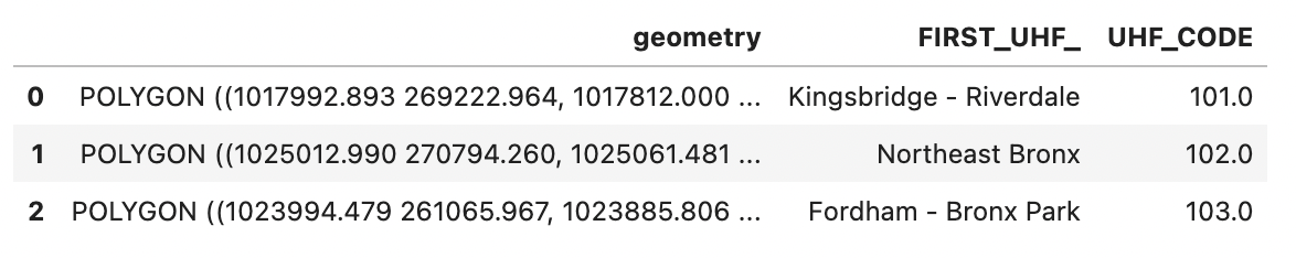
ngbhoods is a GeoPandas GeoDataFrame containing the shapely polygons that define the 35 New York U neighborhoods as defined by the United Hospital Fund, as well as their names and unique ID codes.

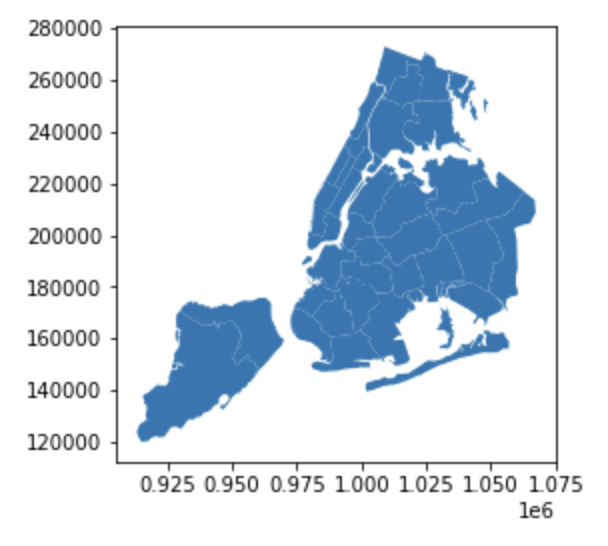
A neat trick to know about GeoPandas is that calling .plot() on a GeoDataFrame will automatically plot the geometries of the shapes contained:

ngbhoods.plot()

When joining spatial datasets, it’s important to standardize the Coordinate Reference System (CRS). A CRS defines how coordinates (numbers like 42.01 or 180000) map to points on the surface of the Earth. Discussing why you’d pick a particular CRS is out of scope for this post, but you visit these links to learn more. What is important is that the two datasets you want to join together have the same CRS. Joining datasets with mismatched CRSs will lead to incorrect results downstream.

The NYC TLC data uses latitude and longitude, with the WGS84 datum, which is the EPSG 4326 coordinate reference system. Let’s inspect the CRS of our ngbhoods GeoDataFrame:

ngbhoods.crs
<Derived Projected CRS: EPSG:2263>

The CRSs don’t match, so we’ll have to transform one of them. It’s more efficient to transform a smaller rather than a larger dataset, so let’s project ngbhoods to EPSG 4326:

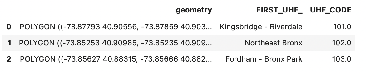
ngbhoods = ngbhoods.to_crs(epsg=4326)

Sidenote: if you are working with multiple GeoDataFrames you can set the CRS of one gdf to that of another using gdf1.to_crs(gdf2.crs) without worrying about the specific CRS numbers.

Calling head() on ngbhoods now will reveal that the values for the geometry column have changed:

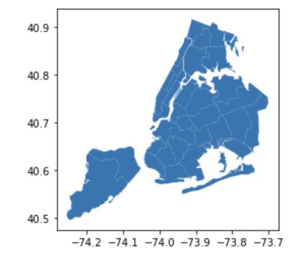
Plotting the GeoDataFrame confirms that our spatial information is still intact. But if you look at the axes, you’ll notice the coordinates are now in degrees latitude and longitude instead of meters northing and easting:

Next, let’s take a look at the regular pandas DataFrame containing our taxi trip data. You’ll notice that this DataFrame also contains geographic information in the pickup_longitude/latitude and dropoff_longitude/latitude columns.

df.head(3)

Looking at the dtypes, however, reveals them to be regular numpy floats:

df.dtypes

vendor_id           object
pickup_datetime      object
dropoff_datetime     object
passenger_count       int64
trip_distance       float64
pickup_longitude    float64
pickup_latitude     float64
rate_code             int64
store_and_fwd_flag   object
dropoff_longitude   float64
dropoff_latitude    float64
payment_type         object
fare_amount         float64
surcharge           float64
mta_tax             float64
tip_amount          float64
tolls_amount        float64
total_amount        float64
dtype: object

Calling plot() on the latitude and longitude columns does not give us a meaningful spatial representation. Let’s see how latitude / longitude values are difficult to interpret without a geospatial library.

Start by plotting the latitude / longitude values:

df.plot(
    kind='scatter', x="pickup_longitude", y="pickup_latitude"
)

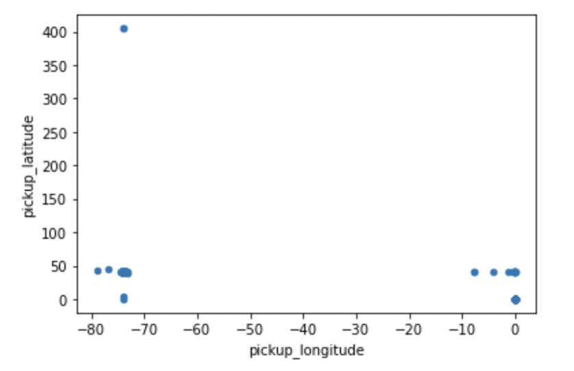
This result is difficult to interpret, partly because there are clearly some data points with incorrect coordinate values in the dataset. This won’t be a problem for our particular use case, but may be worth paying attention to if you’re using this data for other analyses.

Let’s turn df into a GeoPandas GeoDataFrame, so we can leverage the built-in geospatial functions that’ll make our lives a lot easier. Convert the separate pickup_longitude and pickup_latitude columns into a single geometry column containing shapely Point data:

from geopandas import points_from_xy
# turn taxi_df into geodataframe
taxi_gdf = gpd.GeoDataFrame(
    df, crs="EPSG:4326",
    geometry=points_from_xy(
        df["pickup_longitude"], df["pickup_latitude"]
    ),
)

Take a look at first 3 rows:

taxi_gdf.head(3)

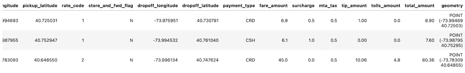
We now have a GeoDataFrame with a dedicated geometry column.

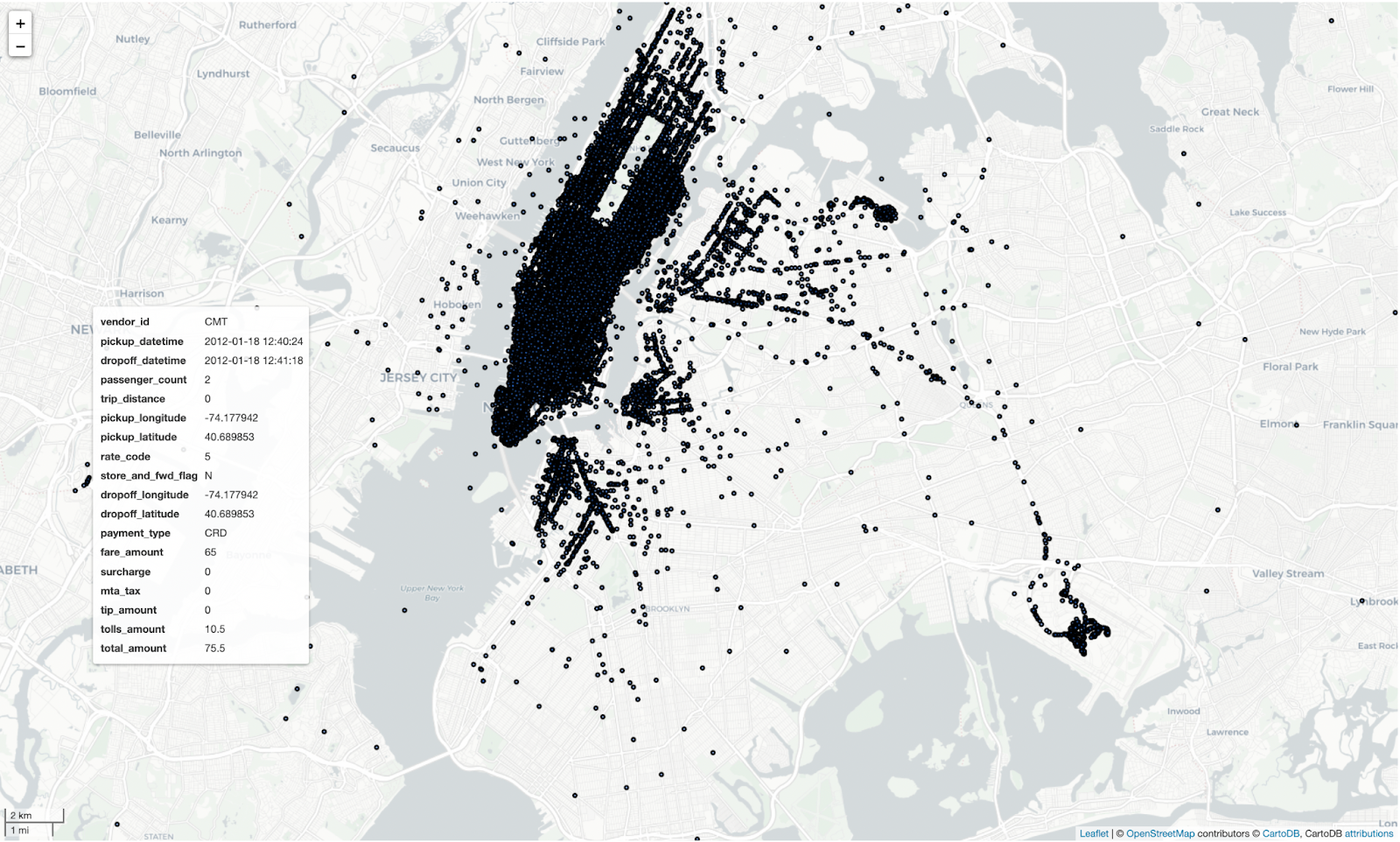
Calling .explore() on a GeoDataFrame allows you to explore the dataset on a map. Run this notebook to interactively explore the map yourself:

taxi_gdf.explore(
    tiles="CartoDB positron", # use "CartoDB positron" tiles
    cmap="Set1", # use "Set1" matplotlib colormap
    style_kwds=dict(color="black") # use black outline
)

Now that both of your datasets have geometry columns, you can perform a spatial join.

Perform a left spatial join with taxi_gdf as the left_df and ngbhoods as the right_df. Setting the predicate keyword to ‘within’ will join points in the left_df to polygons from the right_df they are located within:

%%timeit
joined = gpd.sjoin(
    taxi_gdf, 
    ngbhoods, 
    how='left',
    predicate="within",
)

1.13 s ± 33.3 ms per loop (mean ± std. dev. of 7 runs, 1 loop each)

Clean up and clarify some column names:

# drop index column
joined = joined.drop(columns=['index_right'])

# rename columns
joined.rename(
    columns={"FIRST_UHF_": "pickup_ngbhood_name", "UHF_CODE": "pickup_ngbhood_id"},
    inplace=True,
)

Now that you’ve performed the spatial join, you can analyze spatial patterns in the data.

For example, you can run a groupby that aggregates the mean trip_distance per pickup neighborhood:

res = joined.groupby('pickup_ngbhood_name').trip_distance.mean().sort_values()
res

pickup_ngbhood_name
Rockaway                              18.640000
Southwest Queens                       7.583590
Bayside - Meadows                      5.461818
East New York                          5.195714
Jamaica                                4.933902
Washington Heights - Inwood            4.746627
Pelham - Throgs Neck                   4.478235
Southeast Queens                       4.322500
Kingsbridge - Riverdale                4.140000
Downtown  - Heights - Slope            3.833111
Flushing - Clearview                   3.761765
Sunset Park                            3.612857
Ridgewood - Forest Hills               3.311461
Canarsie - Flatlands                   3.290000
Greenpoint                             3.153171
Long Island City - Astoria             3.055458
Coney Island - Sheepshead Bay          3.036667
West Queens                            3.034350
Central Harlem - Morningside Heights   2.866855
Union Square, Lower Manhattan          2.721932
Bedford Stuyvesant - Crown Heights     2.643019
East Harlem                            2.638558

Spatial Join: Dask-GeoPandas

Now that we’ve seen how to perform a spatial join with GeoPandas, let’s look at how to do the same thing with Dask-GeoPandas. Dask-GeoPandas is particularly useful when you’re working with datasets that are too large to fit into memory.

Let’s load the full NYC TLC dataset for January 2009 (about 120GB of data) into a Dask DataFrame:

import dask.dataframe as dd

ddf = dd.read_csv(
    "s3://nyc-tlc/trip data/yellow_tripdata_2009-01.csv",
    storage_options={"anon": True, "use_ssl": True},
)

Let’s perform some basic data cleaning and filtering:

# convert datetime columns
ddf["pickup_datetime"] = dd.to_datetime(ddf["pickup_datetime"])
ddf["dropoff_datetime"] = dd.to_datetime(ddf["dropoff_datetime"])

# filter out invalid coordinates
ddf = ddf[
    (ddf["pickup_longitude"] != 0) & 
    (ddf["pickup_latitude"] != 0) &
    (ddf["pickup_longitude"].between(-74.3, -73.7)) &
    (ddf["pickup_latitude"].between(40.5, 40.9))
]

Let’s also load some public health data at the neighborhood level:

health = gpd.read_file(
    "../data/CHS_2009_DOHMH_2010B.shp"
)[["geometry", "FIRST_UHF_", "UHF_CODE"]]
health = health.rename(columns={"FIRST_UHF_": "nhbd_name", "UHF_CODE": "nhbd_id"})
health = health.to_crs(epsg=4326)

Now let’s convert our Dask DataFrame into a Dask-GeoPandas GeoDataFrame:

import dask_geopandas

ddf = dask_geopandas.from_dask_dataframe(
    ddf,
    geometry=dask_geopandas.points_from_xy(ddf, "pickup_longitude", "pickup_latitude"),
)
ddf = ddf.set_crs(4326)

Before we perform the spatial join, we need to make sure all workers have access to the health data:

from dask.distributed import Client
client = Client()

# broadcast health data to all workers
health_future = client.scatter(health)

Now we can perform the spatial join:

%%time
joined = ddf.sjoin(health_future, predicate="within")

The spatial join is now distributed across all workers in the cluster. Let’s compute some statistics:

%%time
stats = joined.groupby("nhbd_name").agg({
    "trip_distance": "mean",
    "fare_amount": "mean",
    "tip_amount": "mean",
    "passenger_count": "mean"
}).compute()

This will give us average trip statistics per neighborhood, which we can use to analyze patterns in the data.

Spatial Join: the Final Verdict

• Spatial joins are powerful because they allow you to join datasets based on geographic data.

• GeoPandas is great for performing a spatial join on datasets that fit into memory.

• Dask-GeoPandas scales GeoPandas for larger-than-memory datasets using the parallel processing power of Dask.

• You can speed up a spatial join by running your computations in the cloud using a Coiled Cluster.

	GeoPandas	Dask-GeoPandas	on Coiled
Perform Spatial Join
Support Geographic Data
Parallel Processing
Larger-than-memory Datasets
Scale to the cloud