Large Scale Geospatial Benchmarks: First Pass

Summary

We implement several large-scale geo benchmarks. Most break. Fun!

This article describes those benchmarks, what they attempt, how they break, and the technical work necessary to make them run smoothly.

Context

Last month we published Large Scale Geoscience: Solicitation a community call for geo benchmarks that reflected common workloads in the 100 TiB range. We wanted to source benchmarks that were simple enough to understand, complex enough to be real, and generally very big.

 

Many people contributed to this lively GitHub discussion. Since then we’ve implemented several of those benchmarks and looked at how they run at scale. This post walks through the benchmarks implemented so far, how they perform at scale, and outlines directions for future improvement.

Now let’s go through what has been implemented so far, benchmark by benchmark.

Rechunking

Many applications’ performance depends strongly on data layout. Data laid out in one way (for example partitioned by time) may be inefficient for certain applications (like querying all data at a specific location) and vice versa. To resolve this we often rechunk datasets to have a more friendly structure for the computation at hand.

Rechunking from time-slice partitioned to spatially partitioned

This rechunking benchmark rechunks the ERA5 global climate reanalysis dataset from time-oriented chunks to spatial chunks. This rechunking pattern frequently occurs with Earth Observation (EO) data. Additionally, in this benchmark Xarray/Dask automatically chose to increase chunk sizes from 4 MiB to 100 MiB, which works better with cloud storage.

However, as this workflow scales up we encounter the following issues:

• Large task graphs: As the data volume increases, the graph size increases, resulting in two issues:

  • Initial Delay: Sending the large graphs from the client to the cluster scheduler can take minutes. This is bad both because workers idle during this time, and also because users are confused why there isn’t any progress. This delay is psychologically uncomfortable.

  • Scheduler Memory: Each task takes up about 1kB in RAM. Normally this is fine, but as graph sizes climb to hundreds of millions this can require schedulers with more memory. This is fine in principle (it’s easy to get bigger schedulers) but it’s a common stumbling point for beginners.

• Right-sizing disk size

  • Historically, rechunking used to require a large amount of memory. This was a common pain point for novice users. Fortunately, this has been fixed and Dask array’s newer rechunking algorithm (made default just last month) now uses disk efficiently.

  • Today we’re running out of disk because these benchmarks are so large. This was easy to fix (we can ask either for more workers, or for more storage per worker) but this is a stumbling point for beginners, or those for whom configuring distributed clusters is hard.

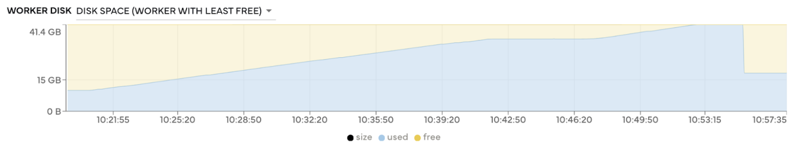
Cluster running out of disk space and crashing.

These challenges of large graph sizes and right-sizing clusters are common concerns to anyone familiar with these tools at this scale. We’re not surprised to see them in a large rechunking workload like this. There are workarounds here that experts use. We’re intentionally not invoking those workarounds. We’re looking forward to working to remove these concerns in a way that will impact less-sophisticated users.

Climatology

Calculating climatologies or seasonal averages is a standard operation when working with weather/climate data. Climatologies are both useful in their own right and also in related computations like anomalies (deviations from the average).

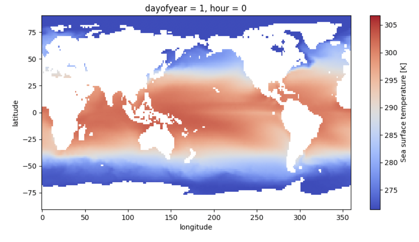
One slice of ERA5 to form a climatology

This climatology benchmark computes seasonal averages of the ERA5 global climate reanalysis dataset. There are a couple of ways to do this.

Ideally we would just write down normal Xarray code, but that fails hard. Instead it has become common-place for users to rechunk the data to align with the climatology one wants to compute, and then do full-chunk calculations. This approach scales better, but also fails. There’s some work to do here as we scale up.

• Weighted rolling reductions scale poorly in Xarray (see this issue for more details).

  Chunk sizes unexpectedly grew from MBs to GBs, which can cause out-of-memory errors.

• Rechunking feels unnatural

  This type of computation today is often reframed using Xarray’s map_blocks as a workaround for the poor rolling performance. However, this approach is tedious and can feel unnatural, especially for less sophisticated Xarray users.

• Anomalies keep data in memory

  This workload is often combined with calculating anomalies. When combining these two we find that Dask doesn’t know if it should drop intermediate data that is used twice (first for calculating the average, and then again for calculating the anomaly) or keep it. This results in a lot of disk engagement, which can be slow, especially on older versions of Dask.

NetCDF to Zarr

NetCDF data is ubiquitous, but often slow and expensive to access in the cloud. Because of this, people commonly convert netCDF data to Zarr, a cloud-optimized format. These workflows often also include a modest rechunking step to improve chunking for cloud access (cloud systems tend to prefer larger reads than POSIX filesystems).

This cloud-optimization benchmark processes the NASA Earth Exchange Global Daily Downscaled Projections (NEX-GDDP-CMIP6) dataset (which is stored as thousands of NetCDF files) by loading the dataset with Xarray, rechunking from time-oriented chunks to spatial chunks, and then writing the result to a Zarr dataset.

See https://cmip6.surge.sh/discoveries/crossingyear/global

As this workflow scales up, we encounter the following issues:

• Xarray’s open_mfdataset doesn’t scale well when reading many files.

  • Xarray today mostly calls open_dataset many times, and then concatenates those results. You’d think that would work well, but it doesn’t. The resulting task graph ends up being a bit unnatural. We can address this by writing a bit of custom code for open_mfdataset

  • It can take non-trivial time to read the metadata of all the NetCDF files. Advanced users know to work around this with the parallel=True keyword argument, which parallelizes the metadata reading on the workers. Unfortunatley, novice users stumble on this.

• As above, this workload inherits the issues around rechunking and right-sizing clusters.

Improving how xarray.open_mfdataset performs on several thousand files will have a broad impact beyond this benchmark on any large scale workload processing data formats like NetCDF.

Atmospheric circulation

This atmospheric circulation benchmark, proposed by Deepak Cherian, computes an Eulerian mean, depending on windspeed and temperature variables.

zonal_means = ds.mean("longitude")
anomaly = ds - zonal_means

anomaly["uv"] = anomaly.U * anomaly.V
anomaly["vt"] = anomaly.V * anomaly.T
anomaly["uw"] = anomaly.U * anomaly.W

temdiags = zonal_means.merge(anomaly[["uv", "vt", "uw"]].mean("longitude"))

This benchmark runs smoothly in small memory (mostly), but graph generation time is painfully slow, waiting almost ten minutes before anything happens.

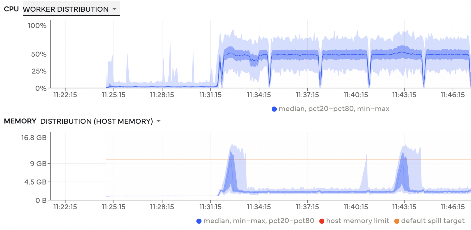
Worker CPU and Memory usage. There’s a long delay before anything occurs.

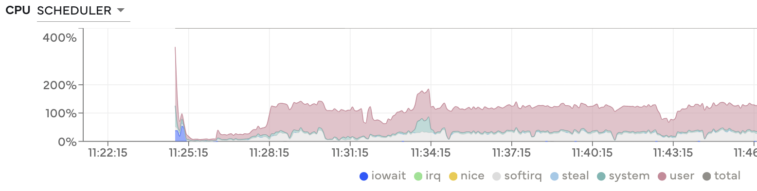
During this period the scheduler is very busy.

All of this points to an inefficiently constructed task graph.

Regridding

Regridding, or remapping, is another common operation when working with geospatial data. It is the process of interpolating data when changing the underlying grid. This may involve a change in the grid resolution or transitioning to a different type of grid. To complicate matters, there is no single standard regridding library people seem to rely on. To learn more about the state-of-the-art, see Max Jones’ Pangeo Showcase. For our benchmark, we have chosen xESMF, which appears to be somewhat common.

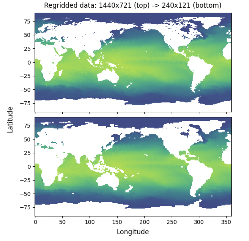
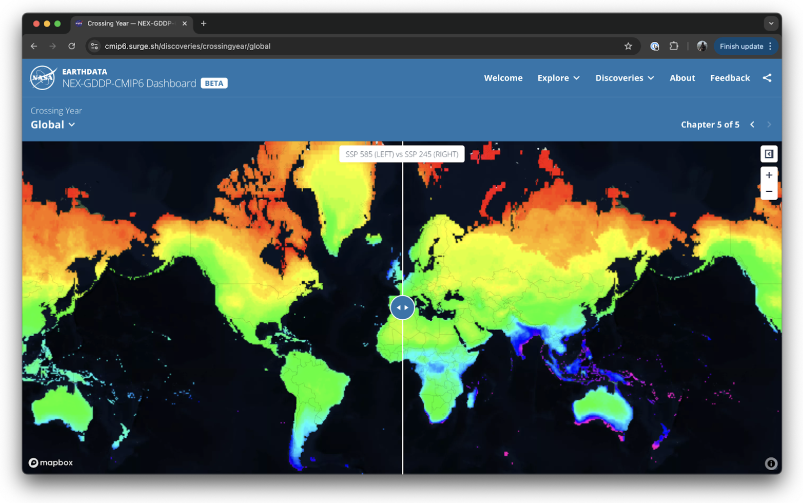
Regridded dataset between fine and coarse resolutions

While this benchmark is embarrassingly parallel along the time dimension, it has problems when scaling the input or output grid due to their effect on the weight matrix used to interpolate the data:

• Sequential Weight Matrix Calculation: The cost of computing the weight matrix is high, and this step precedes the submission of the computation to the cluster. When scaling to higher grid resolutions, this causes the benchmark to stall for minutes before ever submitting work to the cluster, leaving resources underutilized.

• Large Weight Matrices: The size of the weight matrix grows significantly with larger grid sizes. While the matrix for regridding from a 1440×721 resolution to 240×121 takes up around 2 MiB, the matrix for regridding from 1440×721 to 3600×1801 takes up 400 MiB. This matrix is embedded in the task graph, both increasing the size of the graph and the time necessary for submitting it to the cluster.

  Probably we should consider doing this work on the cluster instead.

Satellite Image Processing

Until now most of these benchmarks have been weather/climate/Xarray focused. However, we often encounter completely different use cases and problems in groups mostly focused on satellite imagery. Think of switching out Zarr for COG here.

People working on satellite imagery often don’t need big parallel Xarray jobs, instead they need an easy and efficient way to run a Python function many times on many individual files, each of which fits comfortably in memory. This is common with GeoTIFF data, or with NetCDF files storing L1 or L2 semi-processed satellite data. This user group cares about cloud computing and distributed computing, but the standard challenges around Xarray and Dask don’t apply as strongly.

This benchmark looks through Sentinel-2 data stored on the Microsoft Planetary Computer with the ODC-STAC package, computes a humidity index, and then computes a monthly average.

Additionally we have this historical workload, which lists tens of thousands of small netCDF files, and then does a simple data access computation on each one independently. For this we use coiled.function rather than Xarray (although any serverless function solution should work fine).

@coiled.function()
def process(filename):
    ...

filenames = s3.ls("...")
result = process.map(filenames)

As this workflow scales up, we encounter a different class of issues:

• Limited Availability: We can do lots and lots of work here in parallel, but there are various limits stopping us from getting more workers. We encountered in order:

  • Account quota: the account we were running on had a limited quota

  • Spot availability: as mentioned below, this often becomes a cost optimization game, and even when we had quota we started running out of spot instances

  • Instance type availability: if we’re willing to go beyond spot and pay full price, there are limits to any particular instance type

• Aggressive spinup: it’s not immediately clear how many machines we can use efficiently in parallel.

  By default we’re using Dask’s adaptive scaling heuristics, which run a few tasks and then based on that runtime information scale up accordingly. This is fine, but does mean that it takes a few minutes before the full army of workers arrives, which can be psychologically a little frurstrating. Maybe we can accelerate this a bit and be more aggressive.

This benchmark exposes more about the underlying cloud architecture we use, rather than the open source Python tooling. This makes it a little different than the benchmarks above, but still something that our team is interested in (and we encourage teams of similar deployment projects to take an interest as well). This benchmark is relatively small compared to the others (barely a terabyte) and we’d especially welcome more ideas and contributions in this direction.

GeoPhysical Inversions

Similarly distinct from the Xarray workloads we’ve run into users running thousands of geophysical inversions using SimPEG. This problem is common in mining and resource extraction, or wherever we have sparse measurements within a physically constrained system (is there oil under this rock? Is there water under this soil? Is there cancer under this muscle?). Increasingly as statistical methods become common we find that people want to do not one inversion problem, but thousands, which becomes computationally expensive.

We think that it might be possible to accelerate these workloads with GPUs, so we’re trying that in close collaboration with the SimPEG development team, and teams at NVIDIA. Sorry, no standard benchmark on this one just yet.

Performance Optimization

Once we’ve finished up an initial set of benchmarks (there are still more to do) we’ll start optimizing. This involves running benchmarks, identifying major bottlenecks, and then fixing those bottlenecks wherever we happen to find them in the various open-source projects (Xarray, Dask, s3fs, Zarr, …)

We’ve already identified several areas for improvement above. Let’s list some of them below:

• Moving Large Graphs, which can be resolved both by making our graph representation more compact, or by moving symbolic representations of the graphs instead and expanding them only once they’re on the scheduler.

• Reimplementations of core methods like xarray.open_mfdataset or rolling methods to be a bit more Dask-native where appropriate.

• Better hinting of hardware failures like when rechunking runs out of disk so that users get more sensible error messages and can ask for different hardware

• More aggressive autoscaling so that people feel less compelled to right-size clusters ahead of time and can trust adaptive scaling more (adaptive scaling seems like a nice idea in theory, but most people manually specify sizes still today).

• Well-crafted sane defaults for keywords: Today Xarray experts often specify a mix of keywords when working at larger scales. We hope to be able to replace some of these with heuristics to help more novice users.

• Less reliance on manual rechunking so that users can focus on expressing what they want to compute without worrying about the distributed memory layout or the footprint of individual steps. Instead, Xarray should become better at automatically dealing with chunking schemes that are not optimal.

Feedback

Feedback from the community is critical to ensuring these benchmarks reflect real-world use cases that users care about.

Is this the right set of benchmarks to use? Are key workloads missing?

If you have feedback on these benchmarks or would like to propose a new benchmark, please engage in this GitHub discussion.

Acknowledgments

Finally, thank you to everyone who has engaged in this effort so far. In particular, thank you to Deepak Cherian, Stephan Hoyer, Max Jones, Guillaume Eynard-Bontemps, and Kirill Kouzoubov for contributing benchmarks and discussions.