Nov 21, 2024
4m read
Improving GroupBy.map with Dask and Xarray#
This post was originally published on the Xarray blog.
Running large-scale GroupBy-Map patterns with Xarray that are backed by Dask arrays is an essential part of a lot of typical geospatial workloads. Detrending is a very common operation where this pattern is needed.
In this post, we will explore how and why this caused so many pitfalls for Xarray users in the past and how we improved performance and scalability with a few changes to how Dask subselects data.
What is GroupBy.map?#
GroupBy.map lets you apply a User Defined Function (UDF)
that accepts and returns Xarray objects. The UDF will receive an Xarray object (either a Dataset or a DataArray) containing Dask arrays corresponding to one single group.
Groupby.reduce is quite similar
in that it applies a UDF, but in this case the UDF will receive the underlying Dask arrays, not Xarray objects.
The Application#
Consider a typical workflow where you want to apply a detrending step. You may want to smooth out the data by removing the trends over time. This is a common operation in climate science and normally looks roughly like this:
def detrending_step(arr: DataArray) -> DataArray:
    # important: the rolling operation is applied within a group
    return arr - arr.rolling(time=30, min_periods=1).mean()

data.groupby("time.dayofyear").map(detrending_step)
We are grouping by the day of the year and then are calculating the rolling average over 30-year windows for a particular day.
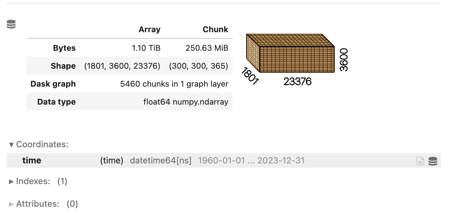
Our example will run on a 1 TiB array, 64 years worth of data and the following structure:

The array isn’t overly huge and the chunks are reasonably sized.
The Problem#
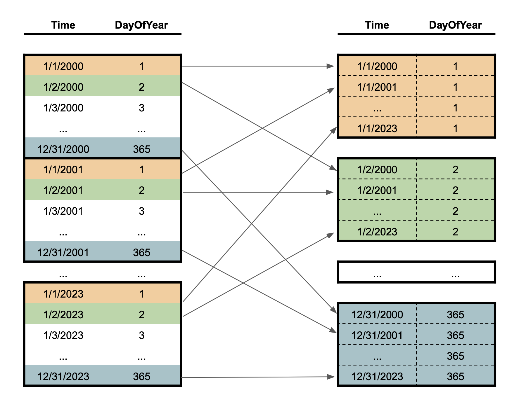
The general application seems straightforward. Group by the day of the year and apply a UDF to every group. There are a few pitfalls in this application that can make the result of this operation unusable. Our array is sorted by time, which means that we have to pick entries from many different areas in the array to create a single group (corresponding to a single day of the year). Picking the same day of every year is basically a slicing operation with a step size of 365.

Our example has a year worth of data in a single chunk along the time axis. The general problem exists for any workload where you have to access random entries of data. This particular access pattern means that we have to pick one value per chunk, which is pretty inefficient. The right side shows the individual groups that we are operating on.
One of the main issues with this pattern is that Dask will create a single output chunk per time entry, e.g. each group will consist of as many chunks as we have year.
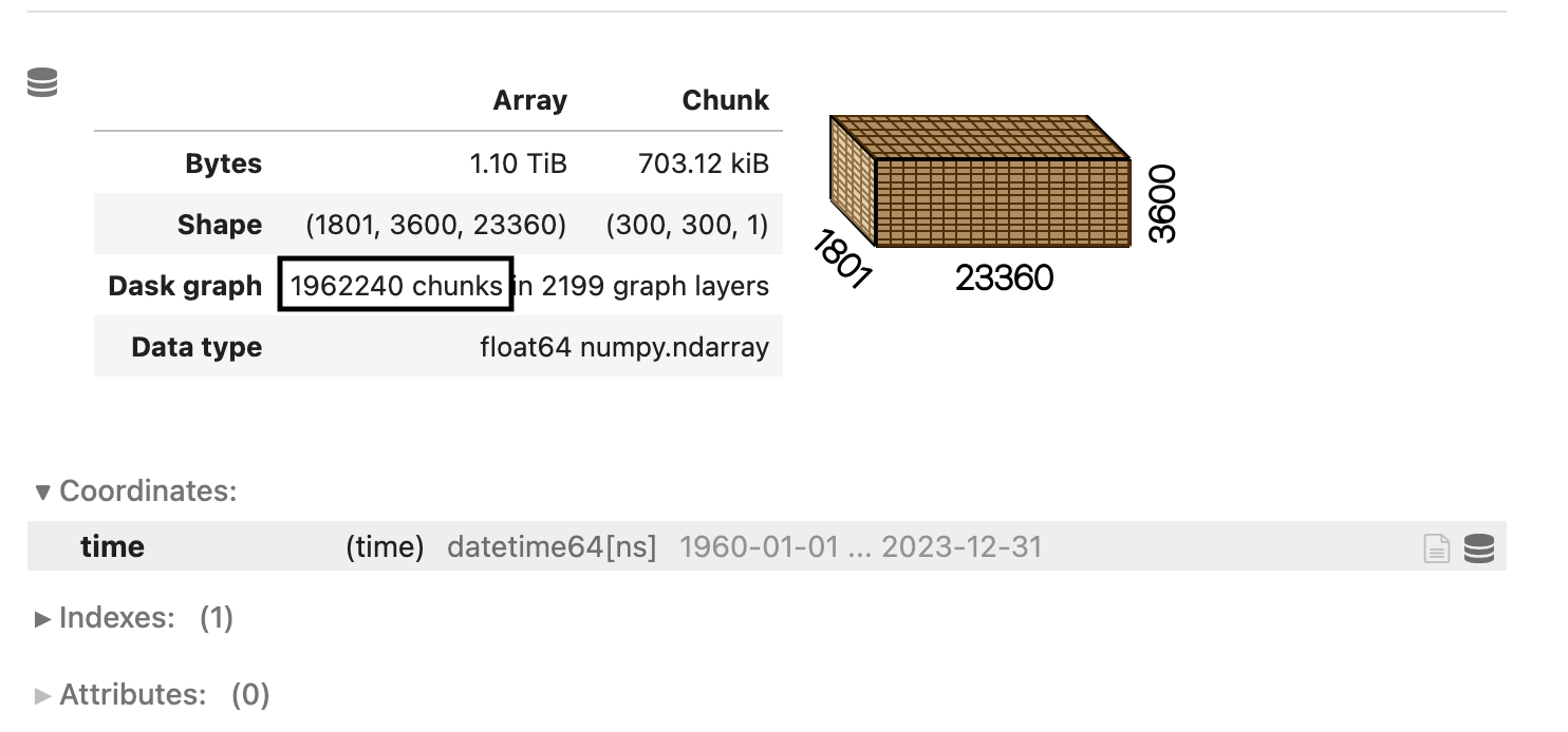
This results in a huge increase in the number of chunks:

This simple operation increases the number of chunks from 5000 to close to 2 million. Each chunk only has a few hundred kilobytes of data. This is pretty bad!
Dask computations generally scale along the number of chunks you have. Increasing the chunks by such
a large factor is catastrophic. Each follow-up operation, as simple as a-b will create 2 million
additional tasks.
The only workaround for users was to rechunk to something more sensible afterward, but it still keeps the incredibly expensive indexing operation in the graph.
Note this is the underlying problem that is solved by flox for aggregations like .mean()
using parallel-native algorithms to avoid the expense of indexing out each group.
Improvements to the Data Selection algorithm#
The method of how Dask selected the data was objectively pretty bad. A rewrite of the underlying algorithm enabled us to achieve a much more robust result. The new algorithm is a lot smarter about how to pick values from each individual chunk, but most importantly, it will try to preserve the input chunksize as closely as possible.
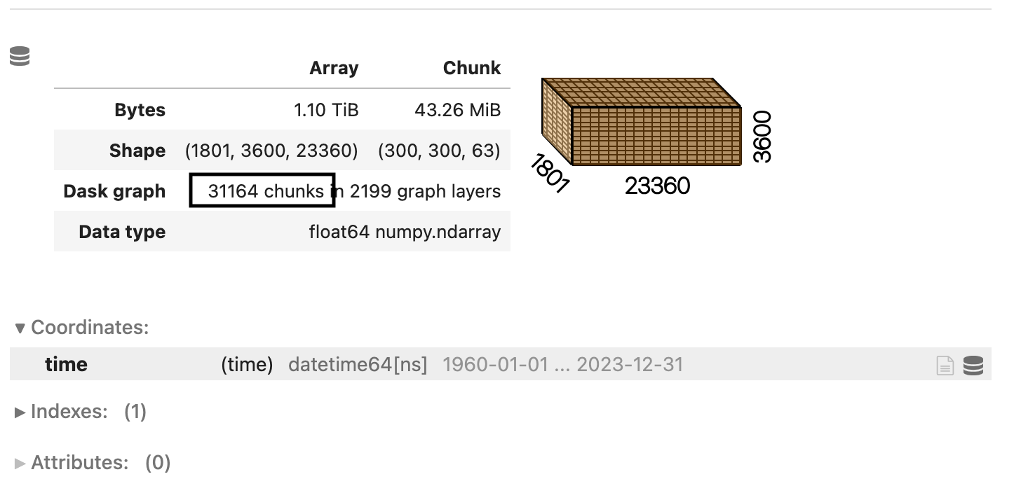
For our initial example, it will put every group into a single chunk. This means that we will end up with the number of chunks along the time axis being equal to the number of groups, i.e. 365.

The algorithm reduces the number of chunks from 2 million to roughly 30 thousand, which is a huge improvement and a scale that Dask can easily handle. The graph is now much smaller, and the follow-up operations will run a lot faster as well.
This improvement will help every operation that we listed above and make the scale a lot more reliably than before. The algorithm is used very widely across Dask and Xarray and thus, influences many methods.
What’s next?#
Xarray selects one group at a time for groupby(...).map(...), i.e. this requires one operation
per group. This will hurt scalability if the dataset has a very large number of groups, because
the computation will create a very expensive graph. There is currently an effort to implement alternative
APIs that are shuffle-based to circumvent that problem. A current PR is available here.
The fragmentation of the output chunks by indexing is something that will hurt every workflow that is selecting data in a random pattern. This also includes:
.selif you aren’t using slices explicitly.isel.sortbygroupby(...).quantile()and many more.
We expect all of these workloads to be substantially improved now.
Additionally, Dask improved a lot of things related to either increasing chunksizes or fragmentation of chunks over the cycle of a workload with more improvements to come. This will help a lot of users to get better and more reliable performance.